Proposed Covariate Development for Forecast and Scenario Models
forecast_covariates.RmdThis vignette focuses on developing covariates that could be used in forecast or scenario SR JPE models. We build upon prior work that identified and tested covariates using historical data, and transition to how those covariates could be adapted for use in forecast or scenario scenarios. These covariates have not been implemented and represent one proposal for forecast covariates.
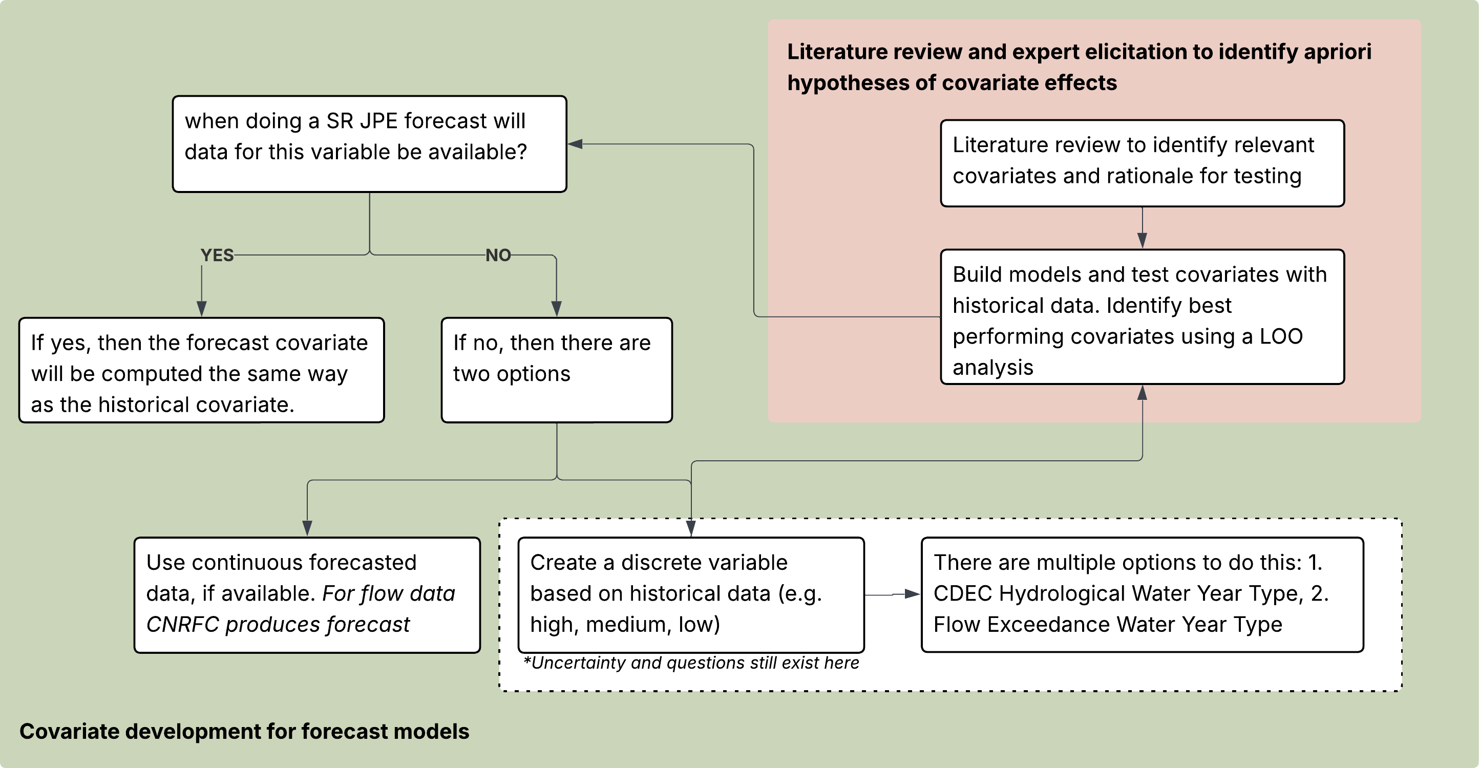
Process for developing forecast covariates
The diagram outlines the process for developing proposed covariates for forecast and scenario models.
Some covariates were selected and evaluated based on literature review and expert input, followed by testing with historical data using leave-one-out (LOO) analysis.
As we transition to forecast and scenario model application, we need to find out if the data for a given covariate will be available at the time of forecasting. If yes, the covariate will be included in the forecast model using the same structure as the historical covariate. If the answer is no, meaning the covariate data will not be available during the forecaste period, then two strategies are considered:
Use continuous forecast data, if available
Create a discrete covariate based on historical data: restructure and bin the variable into categories based on historical conditions (e.g. high, medium, low)
Proposed covariates included in forecast models
| name | description |
|---|---|
| spawning/incubation minimum flow | Use daily max flows for the spawning/incubation time period (Aug-Dec) and then calculate the minimum. This variable is available for all 4 time periods and would be the same because we are using data from the previous Aug-Dec. |
| spawning/incubation maximum flow | Use daily max flows for the spawning/incubation time period (Aug-Dec) and then calculate the maximum. This variable is available for all 4 time periods and would be the same because we are using data from the previous Aug-Dec. |
| spawning/incubation maximum temperature | Summarizes the weekly maximum temperature for each stream (meaning it finds the max across all sites/subsites) within the spawning period. Note that the Sacramento River temperature data does not currently include a daily maximum so the weekly max is the max of the mean. An annual value is calculated by taking the max of the weekly max. This variable is available for all 4 time periods and would be the same because we are using data from the previous Aug-Dec. |
| above 13C threshold | This covariate is defined as the week of the year when the 7DADM is above 13C. Data are filtered to Mar-Dec because this is the time period where spring run are in the tributaries and may be experiencing temperature stress. Note, we currently do not have max daily temperatures for the Sacramento so mainstem is not included. This variable is available for all 4 time periods and would be the same because we are using data from the previous Aug-Dec. |
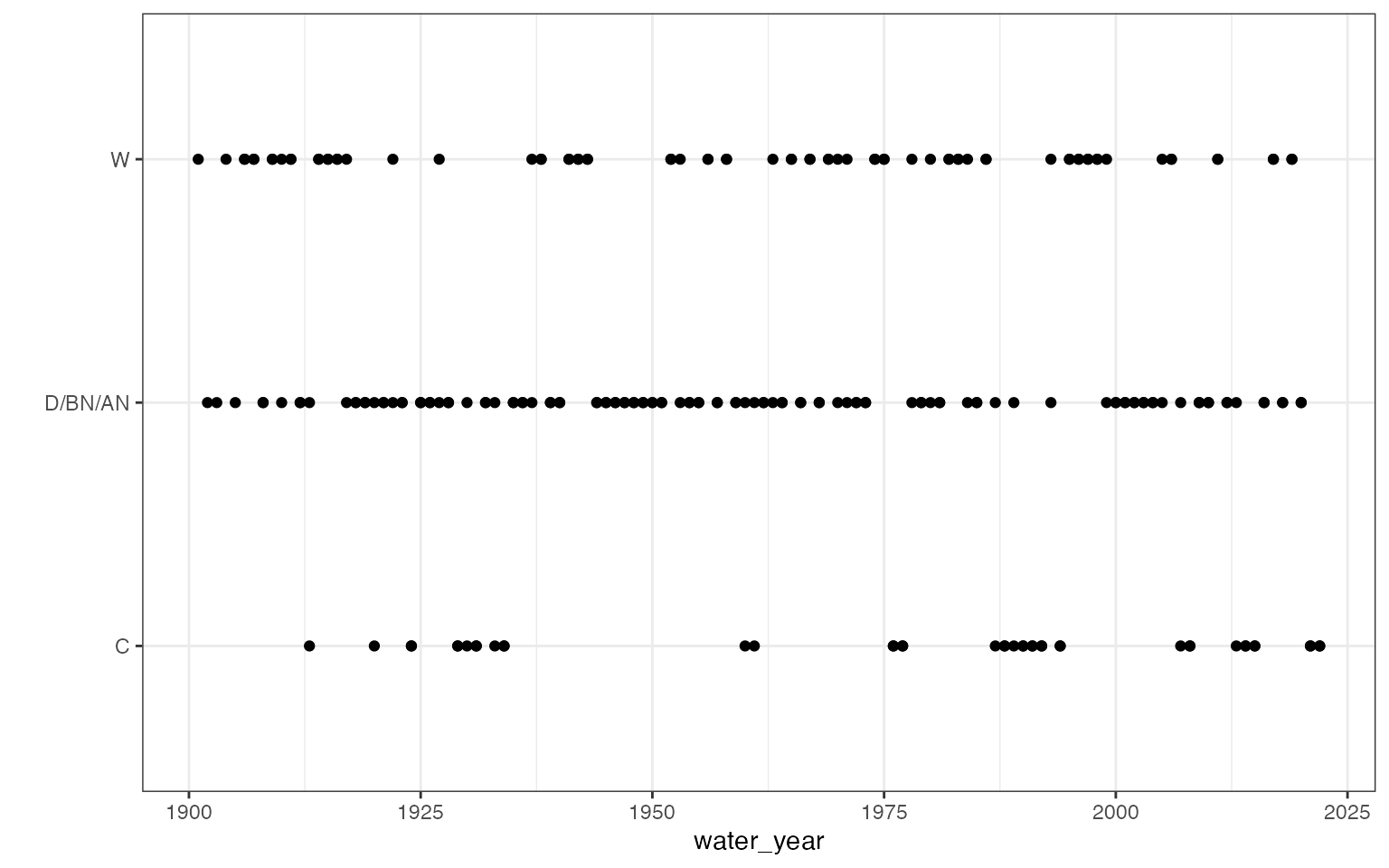
| 3-category water year type | Use water year type from CDEC for the Sacramento Valley and aggregate into 3 categories: C, D/BN/AN, W. This is a scenario based covariate meaning we do not need any data for the forecast. All 3 categories would be run for the forecast. |
| 3-category flow exceedance year type | Use the flow exceedance methodology provided by the CDFW Instream Flow team (find mean annual flow by water year for each stream and rank the water years where the top 33% are wet, middle are average, bottom are dry) to categorize years for each stream into 3 categories: wet, average, dry |
| monthly reservoir storage | Using reservoir storage data, calculate the monthly max storage. For each JPE date we would use data from the month prior (e.g for Jan 1 it would be average for Dec) |
| monthly peak flow | Calculate the peak flow for each watershed and month. This would be different based on JPE date |
Note that this covariate list will be iteratively updated and improved
Preparing covariates
Continuous variables
Spawning and incubation flow variables
These data are pulled from stock_recruit_covarites
- min flow: Use daily max flows for the spawning/incubation time period (Aug-Dec) and then calculate the minimum
- max flow: Use daily max flows for the spawning/incubation time period (Aug-Dec) and then calculate the maximum
Spawning and incubation temperature variables
These data are pulled from stock_recruit_covarites
- max temp: Summarizes the weekly maximum temperature for each stream (meaning it finds the max across all sites/subsites) within the spawning period. Note that the Sacramento River temperature data does not currently include a daily maximum so the weekly max is the max of the mean. An annual value is calculated by taking the max of the weekly max.
- above 13C threshold: This covariate is defined as the week of the year when the 7DADM is above 13C. Data are filtered to Mar-Dec because this is the time period where spring run are in the tributaries and may be experiencing temperature stress. This includes holding as well as spawning and incubation time period.
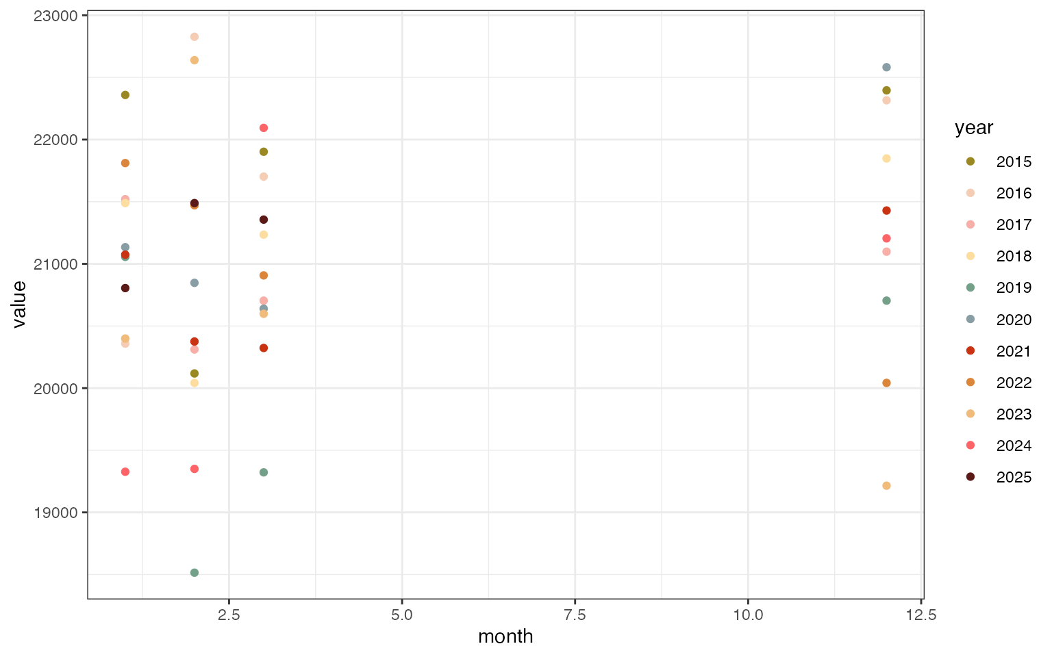
Reservoir storage
- monthly reservoir storage: Using reservoir storage data, calculate the monthly average storage for Keswick Reservoir and Shasta Reservoir. For each JPE date we would use data from the month prior (e.g for Jan 1 it would be average for Dec). This data contains monthly reservoir storage volumes (acre-feet) for Keswick Reservoir (KES), retrieved from the California Data Exchange Center (CDEC) operated by the California Department of Water Resources (DWR) and Shasta Reservoir USGS (11370000).
For Keswick - the earliest data available is in 1965. Stream is NA because it applies to all streams and should not be joined on stream.
For Shasta - the earliest data available is in TODO Stream is NA because it applies to all streams and should not be joined on stream.
Keswick Reservoir (KES)
Plot the last 10 years - note that data have been filtered to Dec-Mar for use in JPE forecasting
Shasta Reservoir (11370000)
Plot the last 10 years - note that data have been filtered to Dec-Mar for use in JPE forecasting
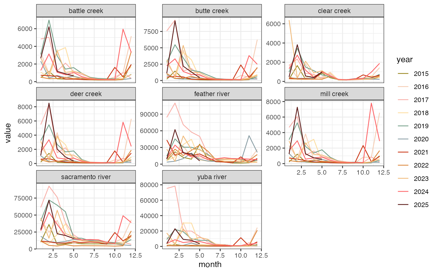
Scenario variales
3-category water year type
- This dataset provides annual Chronological Reconstructed Sacramento and San Joaquin Valley Water Year Hydrologic Classification Indices Based on measured unimpaired runoff (in million acre-feet). It was retrieved from the California Open Data Portal
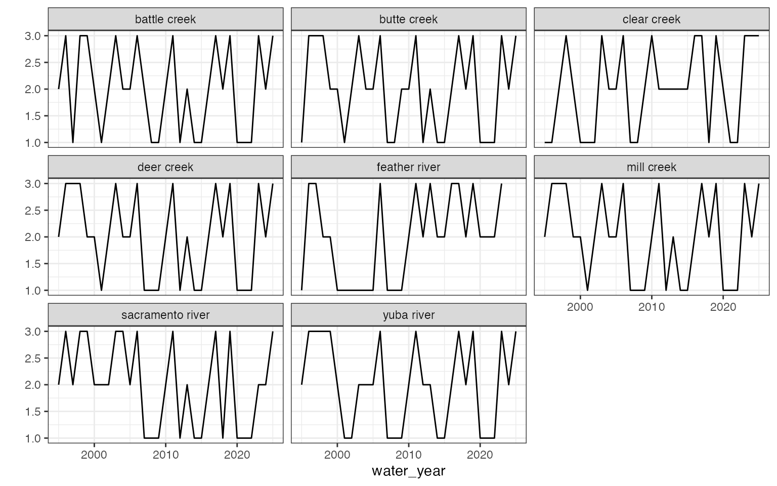
3-category flow exceedance year type
-
This dataset defines the water year type for each stream based on the methodology outlined in the Standard Operating Procedure for Flow Duration Analysis in California CDFW-IFP-005, August 2013. It uses daily flow data from USGS gages to calculate the mean annual discharge (cfs) for each water year and location. Water years are then ranked by mean discharge within each stream and split into three categories:
- Wet: Top 33%
- Average: Middle 33%
- Dry: Bottom 33%

Combine and save data
#> Rows: 6,236
#> Columns: 8
#> $ name       <chr> "si_min_flow", "si_min_flow", "si_min_flow", "si_min_flow",…
#> $ year       <dbl> 1930, 1931, 1932, 1933, 1934, 1935, 1936, 1937, 1938, 1939,…
#> $ water_year <dbl> NA, NA, NA, NA, NA, NA, NA, NA, NA, NA, NA, NA, NA, NA, NA,…
#> $ stream     <chr> "butte creek", "butte creek", "butte creek", "butte creek",…
#> $ value      <dbl> 81, 44, 70, 63, 64, 62, 80, 84, 102, 60, 101, 124, 113, 90,…
#> $ month      <dbl> NA, NA, NA, NA, NA, NA, NA, NA, NA, NA, NA, NA, NA, NA, NA,…
#> $ text_value <chr> NA, NA, NA, NA, NA, NA, NA, NA, NA, NA, NA, NA, NA, NA, NA,…
#> $ site_group <chr> NA, NA, NA, NA, NA, NA, NA, NA, NA, NA, NA, NA, NA, NA, NA,…| name | year | water_year | stream | value | month | text_value | site_group |
|---|---|---|---|---|---|---|---|
| si_min_flow | 1930 | NA | butte creek | 81 | NA | NA | NA |
| si_min_flow | 1931 | NA | butte creek | 44 | NA | NA | NA |
| si_min_flow | 1932 | NA | butte creek | 70 | NA | NA | NA |
| si_min_flow | 1933 | NA | butte creek | 63 | NA | NA | NA |
| si_min_flow | 1934 | NA | butte creek | 64 | NA | NA | NA |
| si_min_flow | 1935 | NA | butte creek | 62 | NA | NA | NA |
| si_min_flow | 1936 | NA | butte creek | 80 | NA | NA | NA |
| si_min_flow | 1937 | NA | butte creek | 84 | NA | NA | NA |
| si_min_flow | 1938 | NA | butte creek | 102 | NA | NA | NA |
| si_min_flow | 1939 | NA | butte creek | 60 | NA | NA | NA |